A collection of geospatial projects built with automated R and Python workflows
Analysis of fire burn severity and post-fire vegetation recovery with Landsat time-series
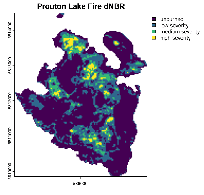
Objective: To examine the burn severity and post-fire vegetation recovery of the Prouton Lake Fire using common vegetative indices (NDVI and NBR) derived from Landsat timeseries data.
Language: R
Project Overview:
- Loaded BC fire polygons and filtered to summarize 2017 fire season statistics and isolate the Prouton Lakes fire boundary
- Looped through all Landsat scenes (2013–2021), cropping to the fire boundary, applying cloud masking, and calculating NDVI and NBR for each scene
- Averaged scene-level indices into yearly composites for both NDVI and NBR
- Calculated dNBR and classified into four burn severity zones, then vectorized into polygons
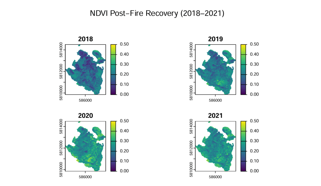
- Masked annual NDVI composites by severity zone (2018–2021) and visualized recovery as maps and boxplots
Packages and Functions:
- sf —
read_sf,st_drop_geometry,st_transform - terra —
rast,crop,mask,app,classify,as.polygons,extract - dplyr / tidyr —
filter,slice_max,pivot_longer,bind_rows - ggplot2
- lubridate / stringr
Code snippet
=====================================================Code snippet from Prouton Lake Fire analysis=====================================================#generate a fire polygon for the Prouton fireprouton_fire_polygon <- fire_polygons %>% filter(FIRE_NO == "C30870") %>% summarise()#list.dirs for Landsat foldersfolders <- list.dirs("data/Landsat 8 OLI_TIRS C2 L2", full.names = TRUE, recursive = FALSE)#create an output directoryout_dir <- "data/output"dir.create(out_dir, showWarnings = FALSE)#create one large for loop to iterate through the folders,#separate files, crop and mask to QA PIXEL, calculate ndvi and nbr, #then save outputs into three separate foldersfor (f in folders) { prod_id <- basename(f) #Extract Date Using lubridate date_string <- stringr::str_sub(prod_id, 18, 25) acq_date <- lubridate::as_date(date_string, format = "%Y%m%d") # Create a clean filename base clean_name <- format(acq_date, "%Y%m%d") files <- list.files(f, full.names = TRUE, pattern = "TIF$", recursive = TRUE) # extract sr + qa files # Select only SR_B1 ... SR_B7 sr_files <- files[grepl("SR_B[1-7]", files)] #build sr stack sr_stack <- terra::rast(sr_files) qa_files <- terra::rast(files[grepl("QA_PIXEL", files)]) # Set CRS and crop rasters to fire polygon prouton_fire_polygon <- st_transform(prouton_fire_polygon, crs(sr_stack)) # crop by polygon and then create the clear mask qa_crop <- terra::crop(qa_files, prouton_fire_polygon, mask = TRUE) clear_mask <- qa_crop == 21824 #crop sr files by polygon, then mask using the clear mask sr_crop <- terra::crop(sr_stack, prouton_fire_polygon, mask = TRUE) sr_mask <- mask(sr_crop, clear_mask, maskvalues = 0) # calculate ndvi and nbr ndvi <- (sr_mask[[5]] - sr_mask[[4]]) / (sr_mask[[5]] + sr_mask[[4]]) nbr <- (sr_mask[[5]] - sr_mask[[7]]) / (sr_mask[[5]] + sr_mask[[7]]) # create directories sr_dir <- file.path(out_dir, "SR") ndvi_dir <- file.path(out_dir, "NDVI") nbr_dir <- file.path(out_dir, "NBR") dir.create(sr_dir, showWarnings = FALSE) dir.create(ndvi_dir, showWarnings = FALSE) dir.create(nbr_dir, showWarnings = FALSE) # write with date writeRaster(sr_mask, file.path(sr_dir, paste0(clean_name,"_SR.tif")), overwrite = TRUE) writeRaster(ndvi, file.path(ndvi_dir, paste0(clean_name,"_NDVI.tif")), overwrite = TRUE) writeRaster(nbr, file.path(nbr_dir, paste0(clean_name,"_NBR.tif")), overwrite = TRUE)
Supervised Image Classification of Land Cover on the Southern Gulf Islands
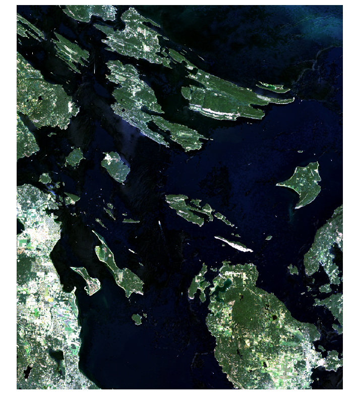
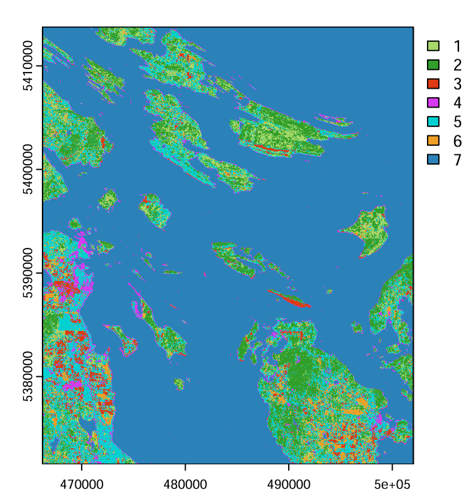
Objective: Perform a supervised land cover classification using Landsat 9 imagery, applying the Maximum Likelihood algorithm to distinguish seven land cover classes and assess classification accuracy.
Language: R
Project Overview:
- Loaded a 6-band Landsat 9 surface reflectance image and delineated 100+ training polygons across seven land cover classes
- Split polygons into 70/30 training and validation sets, extracted pixel-level spectral values, and visualized spectral signatures across all six bands per class
- Ran a Maximum Likelihood classification using
superClass()from RStoolbox, sampling 500 pixels per class to balance training data and reduce bias toward dominant classes like Water - Generated a confusion matrix from validation predictions and calculated Overall Accuracy, User Accuracy, and Producer Accuracy per class
Packages and Functions
RStoolbox— Maximum Likelihood supervised classification and accuracy assessment (superClass)caret— confusion matrix generation and accuracy metric calculation
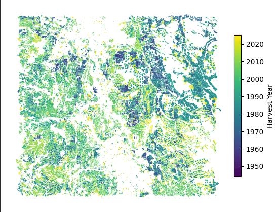
Geospatial Terrain Assessment of Cutblocks in Central BC
Objective: Characterize the topographic conditions of historic harvested cutblocks in central BC, and explore how terrain and hydrologic zones relate to harvesting patterns and geohazard risk
Language: Python
Project Overview:
- Derived slope, aspect, elevation, and curvature rasters from a 30m DEM using
arcpy.sa(Slope, Aspect, Curvature tools) - Calculated per-cutblock mean and standard deviation for each terrain metric using
ZonalStatistics - Cleaned and renamed zonal statistics outputs, then merged all four terrain tables into a single master dataframe joined to the cutblocks geodataframe
- Classified cutblocks into four slope categories (Gentle 0–15°, Moderate 15–30°, Steep 30–45°, Very Steep >45°) based on BC slope classification standards, and summarized total harvested area per class
- Clipped BC Hydrologic Zones to the AOI, then spatially joined zones to cutblocks using to enable zone-level terrain comparisons
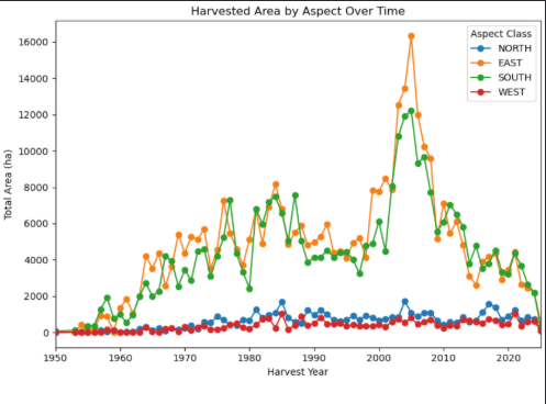
- Visualized temporal harvesting trends and zone-level terrain distributions using
matplotlibandseaborn, including slope over time, mean slope and curvature by hydrologic zone, and the top 10 steepest and largest cutblocks per zone
Packages and Functions
arcpy—Slope,Aspect,Curvature,ZonalStatistics,Clipsimpledbf—Dbf5- pandas /
geopandas—sjoin,merge,groupby,cut matplotlib.pyplot—subplots,figure,showseaborn—barplotos—chdir,path.join,path.splitext,path.basename
Code snippet
#STEP 1: Import libraries
import os
import arcpy
from arcpy.sa import ZonalStatisticsAsTable
import geopandas as gpd
import pandas as pd
import matplotlib.pyplot as plt
import seaborn as sns

#Set up workspace
arcpy.CheckOutExtension("Spatial")
arcpy.env.workspace = os.chdir(r"data\scratch")
arcpy.env.overwriteOutput = True

#STEP 2: Calculate aspect, slope, curvature from dem

dem = r"dem.tif"

#calculate slope
slope_output = arcpy.sa.Slope(
        in_raster= dem,
        output_measurement="DEGREE")
slope_output.save(r"slope.tif")

#calculate aspect
aspect_output = arcpy.sa.Aspect(
    in_raster = dem)
aspect_output.save(r"aspect.tif")

#calculate curvature
curvature_output = arcpy.sa.Curvature(
        in_raster = dem,
        z_factor = 1)
curvature_output.save(r"curvature.tif")

#STEP 3: calculate zonal statistics by cutblock

zone_field = "BLOCK_ID"
output_folder = r"scratch\Outputs"

elev = r"dem.tif"
slope = r"slope.tif"
aspect = r"aspect.tif"
curv = r"curvature.tif"

#function for calculating mean and standard deviation using zonal statistics
def zonal_stats(raster, out_name):

    out_mean_std = fr"{output_folder}\{out_name}_mean_std.dbf"
    ZonalStatisticsAsTable(
        in_zone_data=cutblocks,
        zone_field=zone_field,
        in_value_raster=raster,
        out_table=out_mean_std,
        statistics_type="MEAN_STD",
        ignore_nodata="DATA"
    )

# Run for all four rasters
zonal_stats(elev,  "zstats_elevation")
zonal_stats(slope, "zstats_slope")
zonal_stats(aspect, "zstats_aspect")
zonal_stats(curv,  "zstats_curvature")

#STEP 4: clean up zonal statistics tables and rename fields for better merging
folder = output_folder

# list of (filename, layername) pairs
tables = [
    ("zstats_elevation_mean_std.dbf", "elev"),
    ("zstats_slope_mean_std.dbf",     "slope"),
    ("zstats_aspect_mean_std.dbf",    "aspect"),
    ("zstats_curvature_mean_std.dbf", "curv")]

cleaned = {}  # store cleaned dfs

for filename, layer in tables:
    path = os.path.join(folder, filename)

    # Load DBF into a pandas DataFrame
    dbf = Dbf5(path)
    df = dbf.to_dataframe()

    # Drop unnecessary columns
    df = df.drop(columns=["OID", "COUNT", "AREA"], errors="ignore")

    # Rename MEAN and STD to layer-specific names
    df = df.rename(columns={
        "MEAN": f"{layer}_mean",
        "STD":  f"{layer}_std",
        "HARVEST__!": "HARVEST_YEAR"})

    cleaned[layer] = df

# Merge all cleaned dfs on BLOCK_ID
master = cleaned["elev"] \
            .merge(cleaned["slope"], on="BLOCK_ID") \
            .merge(cleaned["aspect"], on="BLOCK_ID") \
            .merge(cleaned["curv"], on="BLOCK_ID")

#STEP 5: classify by slope angle and plot
cutblocks_gdf = gpd.read_file(cutblocks)

# Merge zonal stats master table
df = cutblocks_gdf.merge(master, on="BLOCK_ID", how="left")

#group by Harvest year 1
df.groupby("HARVEST_YEAR").agg({
    "elev_mean": ["mean", "std"],
    "slope_mean": ["mean", "std"],
    "aspect_mean": "mean",
    "curv_mean": "mean"})

#create slope class bins based on BC slope classification
bins = [0, 15, 30, 45, 90]
labels = ["Gentle (0–15°)", "Moderate (15–30°)", "Steep (30–45°)", "Very Steep (>45°)"]

#create a slope class dataframe using bins and labels described above
df["slope_class"] = pd.cut(df["slope_MEAN"], bins=bins, labels=labels, right=False)

#group by slope class and total area harvested
area_by_class = df.groupby("slope_class")["AREA_HA"].sum()

#plot graphs side by side
fig, axes = plt.subplots(1, 2, figsize=(16, 6))

#plot slope class by total area harvested
area_by_class.plot(kind="bar", ax=axes[0])
axes[0].set_ylabel("Total area harvested (ha)")
axes[0].set_xlabel("Slope Class")
axes[0].set_title("Slope classes of harvested cutblocks by total area")

#plot average slope of harvested blocks over time
(df.groupby("HARVEST_YEAR")["slope_MEAN"].mean()
   .plot(kind="line", ax=axes[1]))

axes[1].set_ylabel("Average Slope (deg)")
axes[1].set_xlabel("Harvest Year")
axes[1].set_title("Average Slope of Harvested Blocks Over Time")
axes[1].set_xlim([1950, 2025])
plt.show()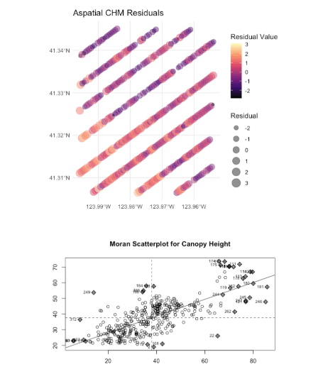
Estimating Canopy Height from Spaceborne Lidar and Sentinel-2 Data Using Statistical Methods
Objective: To model wall-to-wall canopy height across Redwood National Park by integrating GEDI spaceborne LiDAR footprints with Sentinel-2 multispectral imagery, addressing GEDI’s non-continuous spatial coverage to support carbon inventory estimation
Language: R
Project Overview:
- Downloaded and preprocessed GEDI LiDAR footprints and Sentinel-2 multispectral imagery for Redwood National Park, extracting band reflectance values for each GEDI shot location
- Calculated ten spectral indices (NDVI, NDWI, NDMI, EVI, SAVI, NDRE, NBR, GSAVI, and others) from Sentinel-2 bands and assessed correlation with GEDI canopy height via a correlogram
- Ran stepwise AIC selection to identify a six-predictor OLS model, then removed predictors after VIF testing flagged multicollinearity, yielding a stable three-predictor model
- Tested OLS residuals for spatial autocorrelation which confirmed significant autocorrelation and violation of the independence assumption
- Fitted and compared five spatial models Trend Surface, GLS, GWR, Spatial Lag, Spatial Error
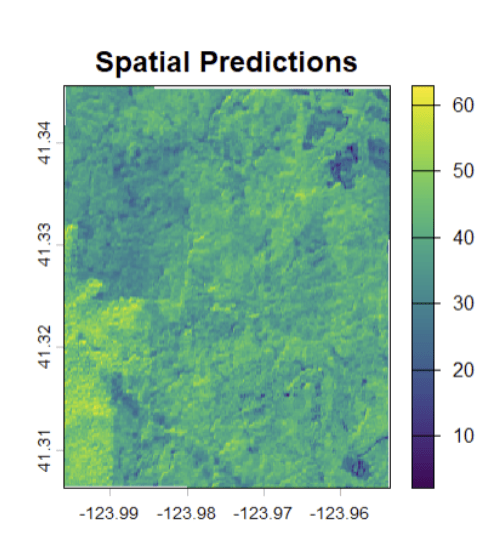
- Selected GLS as the final model based on its stability and interpretability
- Predicted wall-to-wall canopy height across the park using the GLS model and Sentinel-2 imagery, producing a continuous CHM to support carbon inventory estimation
Packages and Functions:
corrplot—corrplotMASS—stepAICcar—vifspdep—knn2nb,knearneigh,nb2listw,moran.test,moran.plot,sp.correlogramgstat—variogram,fit.variogram,vgmnlme—gls,corSpher,residualsspgwr—gwr.sel,gwrspatialreg—lagsarlm,errorsarlmtstats—lm,rstandard,residuals,hist,shapiro.test,AIC,BIC,cor
Code snippet
# Read satellite imagerys2_ras <- rast("data/redwood_aoi_sentinel_2_imagery.tif") # Read AOI datasetaoi <- st_read("data/redwood_aoi.gpkg")# Read our GEDI datagedi_raw <- st_read("data/redwood_gedi.gpkg") %>% # Read GEDI rename(canopy_height = Canopy.Height..rh100.) # Simplify name# Project down to CH & geometrygedi_shots <- gedi_raw %>% dplyr::select(canopy_height)# Preprocessing -----------------------------------------------------------# Extract band information from the Sentinel-2 imagery & convert to DFdf <- terra::extract(s2_ras, vect(gedi_shots), bind=T) %>% st_as_sf()# Output some datadf %>% st_drop_geometry() %>% head()# Add vegetative indices to the data framedf_veg <- df %>% mutate(ndvi = (B8 - B4) / (B8 + B4), ndwi = (B3 - B8) / (B3 + B8), ndmi = (B8 - B11) / (B8 + B11), evi = 2.5 * ((B8 - B4) / (B8 + 6 * B4 - 7.5 * B2 + 1)), savi = ((B8 - B4) / (B8 + B4 + 0.5)) * 1.5, gndi = (B8 - B3) / (B8 + B3), gsavi = ((B8 - B3) / (B8 + B3 + 0.5)) * 1.5, nir_green = B8 / B3, ndre = (B8 - B5) / (B8 + B5), nbr = (B8 - B12) / B8)# View the datadf_veg %>% st_drop_geometry() %>% head()# Aspatial Modelling ------------------------------------------------------# Drop the geometry to investigate correlation between different bands/indicesdf_nogeo <- st_drop_geometry(df_veg)# Calculate & plot correlationdf_cor <- cor(df_nogeo)corrplot(df_cor, method = "color", type = "lower", tl.cex = 0.6, tl.col = "black", addCoef.col = "black", number.cex = 0.4, diag = FALSE)# Use stepwise AIC to create an MLR # Null modelmodel.null <- lm(canopy_height ~ 1,data = df_nogeo)# Full modelmodel.full <- lm(canopy_height ~ .,data = df_nogeo)# Forward selection w/ variables we're interested in model.step <- stepAIC(model.null, direction="forward", scope = list(upper = ~ B3 + B4 + B5 + B7 + B9 + B11 + gsavi, lower = ~1), trace = TRUE)# Check outputssummary(model.step)# Check variable inflation & for co-linearity issuesvif(model.step)#co-linearity issues found for B4# Remove B4 and re-run stepwise AICmodel_final <- stepAIC(model.null, direction="forward", scope = list(upper = ~ B3 + B5 + B9 + B11 + gsavi, lower = ~1), trace = TRUE)# Check modelsummary(model_final)# Check variable inflation & for co-linearity issuesvif(model_final)# Add residuals to check assumptionsdf$resid <- rstandard(model_final)# Check for normalityhist(df$resid)shapiro.test(df$resid)# Check for linearity and independencepar(mfrow = c(2,2))plot(model_final)# Potential independence issues -> # Plot the residuals to investigate for spatial autocorrelationggplot(data = df) + geom_sf(aes(size = resid, color = resid), alpha = 0.5) + scale_color_viridis_c(option = "magma", name = "Residual Value") + theme_minimal() + labs(title = "GEDI Canopy Height Bubbles", size = "Residual", color = "Residual")# Investigate Spatial Autocorrelation -------------------------------------# Use 12 closest neighbours to define neighbourhood structurenb <- knn2nb(knearneigh(df, k = 12))listw <- nb2listw(nb, style = "W")# Test the residuals for spatial autocorrelationmoran.test(df$resid, listw)# Test the canopy height for spatial autocorrelationmoran.test(df$canopy_height, listw)# Create a correlogram to gauge spatial autocorrelationpar(mfrow=c(1,1))plot(sp.correlogram(nb, var = df$canopy_height, order = 10, method = "I", style = "W", randomisation = TRUE, zero.policy = TRUE), main="Moran Correlogram for Canopy Height")# Plot the Moran's I for Canopy Heightgedi_mp <- moran.plot(df$canopy_height, listw) title(main = "Moran Scatterplot for Canopy Height")# Create a bubble plot to investigate spatial autocorrelation of canopy heightggplot(data = df) + geom_sf(aes(size = canopy_height, color = canopy_height), alpha = 0.5) + scale_color_viridis_c() + theme_minimal() + labs(title = "GEDI Canopy Height Bubbles", size = "Height (m)", color = "Height (m)")# Create a variogram for the GEDI canopy heightgedi_vgm <- variogram(canopy_height~1, df, cutoff=2, width = 0.1)# Estimate some initial values for our variogram for fittingpsill <- var(df$canopy_height) * 0.7range <- max(gedi_vgm$dist)nugget <- var(df$canopy_height) * 0.3# Fit the variogram & plotgedi_fit <- fit.variogram(gedi_vgm, model=vgm(psill, "Sph", range, nugget)) plot(gedi_vgm, gedi_fit)# Spatial Modelling -------------------------------------------------------# Add our spatial component as columnsdf_spatial <- df_veg %>% mutate(X = st_coordinates(.)[,1], Y = st_coordinates(.)[,2])# Trend Surface Analysismodel_trend_surface <- lm(canopy_height ~ B3 + B5 + gsavi + X + Y, data = df_spatial)# GLSmodel_gls <- gls(canopy_height ~ B3 + B5 + gsavi, correlation = corSpher(form = ~ X + Y, nugget=TRUE), data=df_spatial)
